Landscape classification using the Atlas of Living Australia

Author: Professor Brendan Mackey, The Fenner School of Environment and Society. The Australian National University

Brendan Mackey

Prof Brendan Mackey,
The Australian National University

Introduction

Our capacity to analyse space and time patterns in biological, ecological and environmental phenomena was transformed in the 1980’s by Geographic Information Systems (GIS), remote sensing and computer-based environmental modelling. In parallel, developments in numeric analysis addressed the ever-growing volume of spatial data. At the forefront of these developments were the pioneering efforts of the CSIRO Division of Land Use Research (now Land and Water), with one of its well-known products being Lee Belbin’s PATN program (Belbin 1989). Within PATN was a suite of functions that provide a flexible approach to the numeric classification of landscapes and seascapes, enabling areas of vast geographic extent to be analysed at increasingly fine spatial resolutions. These capacities broke the pre-digital geographer’s adage that “analysis of large extent means using course resolution data”.

Over the last 20 years the PATN approach has been applied to a large array of research and practical problems, including assessment of World Heritage values in the Wet Tropics of Australia (Mackey et al. 1989), rainforest-environment relationships (Mackey 1993), comparison of boreal forest management ecoregions (Mackey et al. 1996), biodiversity management in New Zealand (Leathwick et al. 2003), and a range of applications in South Africa (Fairbanks 2000) and the USA (Hargroves and Hoffman 2005). One core PATN function that enabled these landscape classifications (Belbin, 1987) have now been incorporated into the Spatial Portal of the Atlas of Living Australia.

Why do we want to classify landscapes?

Classification can be applied to various kinds of biodiversity-related problems and questions. The approach is equally applicable to seascapes but the focus of this Case Study is a terrestrial application. There are three foci of landscape classifications (Mackey et al. 2008):

Patterns in ‘composition’ and ‘evolutionary legacy’ as represented by the taxonomy, phylogeny and genetic structure of plant and animal species. Digitisation of museum and herbarium species location data enables spatial analyses of patterns in species richness and endemism at global, continental and regional scales (Myers et al. 2000; Crisp et al. 2001; Proches 2005; Slatyer et al. 2007). Molecular data provide new information for mapping biogeographical patterns in the phylogeny and genetic structure of taxa and analysis of their environmental relations (Hawkins et al. 2005; Kirchman and Franklin 2007) and modes of speciation (Norman et al. 2007).
Patterns in the drivers of ecosystem processes. These are usually represented by exogenous environmental variables such as climate, water availability and substrate fertility. The mapped spatial patterns were coined by Henry Nix as environmental domains. Applications of environmental domain analysis include identifying regions for the purposes of: (a) “coarse filter” gap analysis (Scott et al. 1993) in systematic conservation planning where the mapped regions are used as ecosystem surrogates (Mackey et al. 1988); and (b) mapping regions within which the landscapes are likely to be amenable to similar conservation and natural resource management guidelines and prescriptions (Hobbs and McIntyre 2005).
Patterns in ecosystem response. Remotely sensed data provide the means to monitor the response of landscape ecosystems to seasonal and year-to-year variation in weather conditions, fire events, land use activities, and climate change. A major ecosystem response which is sensitive to such exogenous factors is gross primary productivity – the rate (integrated over a day, month or year) of photosynthesis (CO₂assimilation) by the vegetation canopy over an area of the Earth’s surface. Time series data are particularly useful as they enable analysis of yearly and seasonal variability in primary productivity (Berry and Roderick 2004; Berry et al. 2007)

What are the benefits of numeric classification?

Prior to the numerical approach, landscape were classified using an ‘Integrated survey’ method whereby spatial units were classified by land surface patterns perceived by an expert through visual interpretation of air-photo images supported by reconnaissance field survey (Christian and Stewart 1968). The mapped patterns largely reflected the expert’s field of knowledge and on-ground familiarity with the region of study. The method therefore lacked a sufficient degree of objectivity and thus repeatability. A fundamental limitation of the integrated survey approach is the assumption that biogeographical entities comprise spatially nested hierarchies, which is not always the case. Furthermore, there was no explicit method for extrapolating the field survey data; correlation of sampled and un-sampled spatial units was assumed.

The numeric approach uses a bottom-up classification procedure – spatial patterns are generated based on analysis of a large number of spatial units such as grid cells or micro-catchments. The spatial units are agglomerated into classes based on a quantitative measure of their biological, environmental or ecological similarity. Classes of regions can be spatially disjunct, adjacent or nested as empirically revealed. This approach has the advantage of forcing theoretical assumptions about how the land is classified to be made explicit, making a classification repeatable.

The Case Study

The Case Study is based on a classification of the Australian continent focused on the second theme above; patterns in the drivers of ecosystem processes.

The Atlas classification option is accessed from the menu option, ‘Tools’ and then ‘Classify’. The study area is selected first; in this case, Australia. Then, the user selects the variables to be used in the classification. The choice of variables should be primarily guided by the purpose of the classification and the nature of the phenomenon being studied. It helps if a specific question is formulated which the classification can address. I was interested in identifying which landscapes in Australia have continentally distinctive substrates that are apparent within major climatic regimes and which may continue to exercise a dominant control on vegetation productivity and structure under a changing climate. In this study, I aimed at using a minimal set of variables: precipitation annual, temperature annual minimum mean and fertility based on lithology were selected.

When each variable is selected, a colour code appears in the right hand column; red indicates variables (environmental layers) which are highly correlated with any of the already-selected variables, green indicates low correlation and yellow as intermediate. Selecting multiple variables with high correlation will unduly weight that environmental component.

The next step is to select the number of groups to be generated by the classification. Here I specified 50. The spatial data layers I used in the classification have a ~1km grid cell resolution. The classification tool allocates the grid cells to groups based on the similarity of all of their attribute values. The final step is to name the new classification layer that will be produced.

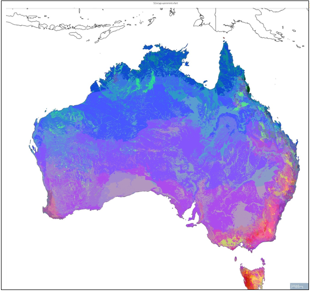
There are two main outputs from the classification. The first is a map showing the classification of the grid cells. The image below shows the map of the 51 group classification. While I specified 50 groups, the program may generate a slightly different number if the selected number is not a stable solution.

Spatial representation of the 51 group environmental domain classification of theAustralian continent generated by the ALA Spatial Portal classification function.

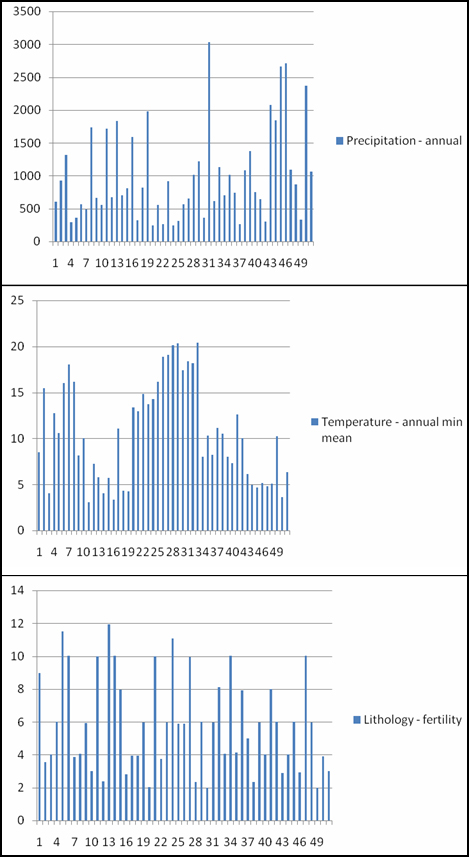
Mean values for the 51 classification groups generate by the numeric classification.

The second main output is a zip file containing a Classification means csv file (comma-separated values) file (zip file 7.4 MB, csv file 3 KB) providing the mean values of (in this case) the three environmental variables for each classification group. This file can be used for additional analyses and diagnostics in statistical packages such as PATN, R or Excel. Using Excel, the group means were plotted as histograms (see image below).

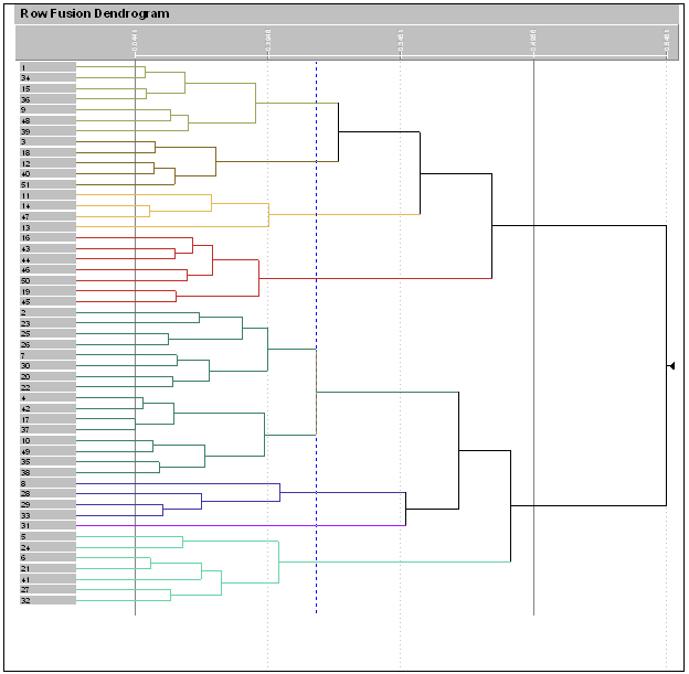
A dendrogram was generated using PATN. A dendrogram displays the hierarchical relationship of the groups based on a measure of their inter-group similarity (see image below).

A dendrogram showing the inter-group similarity of the 51 groups (environmental domains generated by the continental classification. The level of similarity delineating the 8 group level is indicated by the dotted line

The classification layer (see top image) uses group colours based on group differences (Belbin et al. 1983).

The choice of the number of classification groups is subjective but the following heuristics can be applied: (i) chose a larger number by a factor of 2-3 than what you think you will need; (ii) re-run the analyses with a very large and then a very small number of groups; (iii) compare the classification with independent data relevant to the phenomenon being studied, including other regionalisations of the study area; and (iv) use the dendrogram and group means to consider the significance of groups distinguished at different levels of similarity.

Examining the top image, it appears that more of the groups have been assigned where climatic gradients are steepest (e.g. the eastern Ranges, Tasmania, South West W.A.). A smaller proportion of the 51 groups have been assigned to inland Australia, reflecting its low relief, arid conditions and broad thermal gradients. Also apparent is the contrast between the northern summer monsoonal tropics and the so-called Mediterranean (winter rain) climatic domains of southern Australia. Certain soils are also evident in the classification including the carbonate soils (calcarosols) of the Nullarbor Plan and cracking clays (vertosols) of the northern Mitchell Grasslands (see McKenzie et al. 2004). The vegetation structure of these two bioregions is strongly influenced by the role substrate plays in determining soil water availability and soil fertility. It follows that these kinds of variables must be factored into models that aim to predict climate change impacts on Australian ecosystems.

Help on the Classification

See the Spatial Portal Classification (Tools) for more information on how the classify works.

See the Classification Help »

About the author

Brendan Mackey is a professor of environmental science at The Fenner School of Environment and Society, The Australian National University. He has a long standing interest in the application of GIS, remote sensing and environmental modelling to biogeography and biodiversity conservation problems. His current research is focussed on regional planning for biodiversity, connectivity conservation, and the carbon dynamics of forests ecosystems and related policy issues.

Contributors to this page

The Australian National University

Scientific References

Belbin L. (1989) PATN Technical Reference. CSIRO Division of Wildlife and Ecology, Canberra.

Belbin L. (1987) The use of non-hierarchical allocation methods for clustering large sets of data. Australian Computer Journal 19, 32-41.

Belbin L., Marshall C., and Faith D.P. (1983) Representing relationships by automatic assignment of colour. The Australian Computing Journal 15, 160-163.

Berry S., Mackey B. and Brown T. (2007) Potential applications of remotely sensed vegetation greenness to habitat analysis and the conservation of dispersive fauna. Pacific Conservation Biology 13, 120-127.

Berry S. L. and Roderick M. L. (2004) Gross primary productivity and transpiration flux of the Australian vegetation from 1788 to 1988 AD: effects of CO2 and land use change. Global Change Biology 10, 1884-1898.

Christian C.S. and Stewart G.A. (1968) Methodology of integrated surveys. Aerial survey and integrated studies. Conference Proceedings (ed. by UNESCO), pp. 233–280. UNESCO, Toulouse, France.

Crisp M.D., Laffan S., Linda H.P. and Munro A. (2001) Endemism in the Australian flora. Journal of Biogeography 28, 183–198.

Fairbanks D.H.K. (2000) Physio-climatic classification of South Africa’s woodland biome. Plant Ecology, 149, 71–89.

Hargrove W.W. and Hoffman F.M. (2005) Potential of multivariate quantitative methods for delineation and visualization of ecoregions. Environmental Management 34, S39–S60.

Hawkins B.A., Diniz-Filho J.A.F. and Soeller, S.A. (2005) Water links the historical and contemporary components of the Australian bird diversity gradient. Journal of Biogeography 32, 1035–1042.

Hobbs R.J. and McIntyre S. (2005) Categorizing Australian landscapes as an aid to assessing the generality of landscape management guidelines. Global Ecology and Biogeography 14, 1–5.

Kirchman J.J. and Franklin J.D. (2007) Comparative phylogeography and genetic structure of Vanuatu birds: control region variation in a rail, a dove, and a passerine. Molecular Phylogenetics and Evolution 43, 14–23.

Leathwick J.R., Overton J.McC. and McLeod, M. (2003) An environmental domain classification for New Zealand and its use as a tool for biodiversity management. Conservation Biology 17, 1612–1623.

Mackey B., Berry S. and Brown T. (2008) Reconciling approaches to biogeographic regionalization: a systematic and generic framework examined with a case study of the Australian continent. Journal of Biogeography 35, 213–229.

Mackey B.G., McKenney D.W., Yang Yin-Qian, McMahon J.P and Hutchinson M.F. (1996) Site regions revisited: a climatic analysis of Hill’s site regions for the province of Ontario using a parametric method. Canadian Journal of Forest Research 26, 333-354.

Mackey B.G. (1993) A spatial analysis of the environmental relations of rainforest structure. Journal of Biogeography 20, 303-356.

Mackey B.G., Nix H.A., Hutchinson M.F., McMahon J.P. and Fleming P.M. (1988) Assessing representativeness of places for conservation reservation and heritage listing. Environmental Management 12, 501-514.

Mackey B.G., Nix H.A., Stein J., Cork E. and Bullen F.T. (1989) Assessing the representativeness of the Wet Tropics of Queensland World Heritage Property. Biological Conservation 50, 279-303.

McKenzie N., Jacquier D., Isbell R. and Brown K. (2004) Australian soils and landscapes: an illustrated compendium. CSIRO Publishing, Collingwood.

Myers N., Mittermeier R.A., Mittermeier C.G., da Fonseca G.A. & Kent J. (2000) Biodiversity hotspots for conservation priorities. Nature 403, 853–858.

Norman J.A., Rheindt F.E., Rowe D.L. and Christidis L. (2007) Speciation dynamics in the Australo–Papuan Meliphago honeyeaters. Molecular Phylogenetics and Evolution 42, 80–91.

Proches S. (2005) The world’s biogeographic regions: cluster analyses based on bat distributions. Journal of Biogeography 32, 607–614.

Scott J.M., Davis F., Csuti B., Noss R., Butterfield B., Groves C., Anderson H., Caicco S., D’Erchia F., Edwards T.C., Ulliman J. Jr. and Wright R.G. (1993) Gap Analysis: A geographic approach to protection of biological diversity. Wildlife Monograph 123, 1-41.

Slatyer C., Rosauer D. and Lemckert F. (2007) An assessment of endemism and species richness patterns in the Australian anura. Journal of Biogeography 34, 583–596.