January 30, 2012
Tabulation is the contextual layer counterpart to Scatterplots. In scatterplots, the X and Y axes are environmental layers (e.g., temperature, rainfall) and the points on the graph are occurrences. With tabulation, contextual layers (e.g., land use, States and Territories) form the X and Y axes as rows and columns of a table and the entries in the table cells are spatial intersections and can be any one of the following 12 values:
- Area of intersection (km2)
- Percentage of area (a)
- Percentage of row total (a)
- Percentage of column total (a)
- Number of species of taxa/assemblage
- Percentage of species of taxa/assemblage (e)
- Percentage of row total of (e)
- Percentage of column total of (e)
- Number of occurrences of selected taxa
- Percentage of occurrences of selected taxa (i)
- Percentage of row total of (i)
- Percentage of column total of (i)
On the ‘Tools menu, select ‘Tabulate’.

Tabulation Step1 chosen values
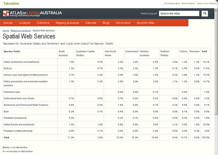
The example is for Species richness (%) tabulated across ‘Australian States and Territories’ for ‘Land cover (class’). The 1.9% is the first row and column of the table is interpreted as 1.9% of species richness in South Australia occurs in ‘Native shrublands and heathlands’. (Click the image below to enlarge.)

Tabulation Screenshot - can download CSV file or open in new window
NOTE: Area tables may contain cells containing “0” (square kilmoetres). Where spatial intersections between the pair of contextual layers produces a small sliver area less than 50% of the smallest grid cell used, the value can be rounded down to zero. The occurrence and species counts will howver be correct.
Click the ‘Download output’ to access the tabular CSV file. A spreadsheet that contains all the formulas for an example tabulation can be found at
A page giving all the combinations of layers and all the different value types with the three different formats – html, csv, json – using Spatial Web Services is also available »
Demonstration Video
(More detail to be added later … RL to note).