Layers are used to overlay both environmental and contextual layers on the map.

To add a new layer, select from the Menu Option, Add To Map | Layers.
This Layers option maps any of the layers available in our Layer Library. On this page, there are a few links to view/download information in the form of a table about each of the layers in the Atlas.
These layers can be viewed, sampled and generally used in analysis but cannot currently be downloaded in raw data form due to licensing constraints. The Atlas has been given most of these layers with an agreement not to pass them on to a third party. The agencies responsible for each layer are listed in the CSV download file along with the license type. When agencies move to Creative Commons licences, we will provide various options to download the layers.
There are two distinct types of layers available:
- Environmental: These are layers that are based on a regular grid. In most cases, the Atlas has aligned a wide range of layers to have the same grid origin, size and orientation. The values of the grid cells are continuous numeric, for example, temperature in degrees centigrade or precipitation in mm. Generally, the environmental layers in the Spatial Portal are included because they are thought by experts to have some control or relationship with the distribution of organisms.
- Contextual: These layers are essentially polygonal even though some are generated on a grid basis. The values within each of the polygons is a class such as “forestry” as a land-use class. Generally, contextual layers are used to interpret the distribution of organisms rather than controlling them in some way, hence the name. Contextual data may also be helpful in interpreting the output of an analysis. For example, what is the distribution of land-use classes where this species is found or could be predicted to be found.

There are three distinct ways to map layers:
- If you know the name of the layer you want, you can start typing the name into the Layer text box. As with species names, the system will know some synonyms (e.g.: rainfall=precipitation). Typing the first three letters will start to bring up a list of matching names. Once a layer name has been clicked, it will be mapped.
- If you do not know the name of the layer you want, you can type in a keyword and the auto-complete feature will suggest possible matches. A list of keywords can be viewed in the layer list. Once a layer name has been clicked, it will be mapped.
- All ~500 (environmental and contextual) layers have been assigned to a 2-level classification. If you want to browse the available layers, use the classification tree.
Layer selection box
The box for selecting layers to map or to use in analysis contains a range of functions. This list and selection box enables you to
- Select one or multiple layers individually from the table using the check boxes. You can map one or any number of available layers at one time. NOTE: Use the Map option box to select or deselect all mapped layers.
- Add set of layers entry box
- Select previously used layers (a list of your most recent layers is kept)
- Select a predefined suite of layers, for example the ‘Best 5’ (see below for details on how these suites are generated).
- Import a list of layer names saved or generated previously. The format uses short-names separated by commas (CSV-format). To see an example of the format, use the fexport option once layers have been selected.
- Add from Search entry box
- Search for a layer using auto-complete (the same type of function as used for species selection, but in the case of layers, the search covers any words in the long name, short name, classification and keywords: See http://spatial.ala.org.au/layers). Just start typing and he auto-complete will start displaying layers that match what you have typed.
- Clear selection deselects any selected layers
- Export layer set creates a text file comtaning the (short-name) list of selected layers. This can be used for subsequent import.

Layers list box
When you first see the layers selection table, you will see
- A link to the list of all available layers. At the time of writing, there are close to 500 layers available.
- The checkboxes for the selection of layers
- The classification of the layers. The classification has two levels as for example ‘Area management’ | ‘Biodiversity’ or ‘Substrate | moisture’.
- The long name of the layer
- A colour. As the text to the left of the layer list suggests, “The colours against the layers are like traffic lights. Green implies the layer is uncorrelated to all selected layers, orange implies some correlation while red implies high correlation. As you select layers, the colours change to reflect correlation with already selected layers. For example a red layer implies high correlation with at least one selected layer while a green layer implies little or no correlation to any selected layer
Note: The correlations are currently based on full layer spatial extents and not any selected sub-area.”
Note: Even though there may be some spatial overlap between terrestrial and marine layers, they are designated as mutually independent suites.
- A clear layers button. This resets any selected layers
- An Export set button that will save the list of selected layers to a CSV file.
The “Next” button will be enabled when at least one layer has been selected.
Layer suites
There are a number of predefined suites of layers that you may find useful for a range of biodiversity applications. In all current suites, the same algorithm has been applied. The philosophy behind the suites is relatively simple – can we identify a subset of all available environmental layers that appear to cover the range of terrestrial environments? The strategy developed (by Lee Belbin in 2011) is related to the traffic light colours noted above:
- Use the inter-layer association matrix (http://spatial.ala.org.au/files/) to generate an (SSH 3d) ordination using http://www.patn.com.au
- Select the layer that is at the extreme end of the spatial distribution as the first of the subset
- Select the layer that is furthest away in the ordination (environmental space) from the first selected layer that also shows the most complementary spatial distribution of values. In some cases, the layer selected may indeed be complementary but also be degenrate in that it may have little or no spatial variation of values over most of the continent. If this is the case, a spatially adjacent layer in the ordination that has a more complementary distribution of values to the first layer is selected.
- Select a third layer that is most somplementary to the both already selected layers (that is also not ‘spatially degerate’).
- Continue the selection of layers until no remaining layer is greater than a respectable (ordination) distance from all selected layers.
Generally, it has been found that 5 layers appear to cover most of the variation in terrestrial environments across the Australian continent.

Layers suite, previous, import selection box
There are currently three predefined suites of layers in the Spatial Portal-
- A suite of the best 5 layers based on bioclim-only layers. These layers are based on the work of Nix, Hutchinson, Stein and others (see http://fennerschool.anu.edu.au/files/panel/448/creswww_pdf_54059.pdf). These layers have names with “Bioxx” where xx are the values 1-35.
- A suite of the best 5 layers of a set of environmental layers provided by Dr Kristen Williams (CSIRO Ecosystems Sciences). These layers are 1960 centred.
- The best 5 2030 equivalents to layers in (2) as provided by Dr Kristen Williams (CSIRO Ecosystems Sciences).
NOTE: If a smaller area was to be used, the inter-layer dissimilarity matrix for all layers would have to be generated. Currently, due to the processing required, the Spatial Portal of the Atlas only generates the association matrix when new environmental layers are added.
NOTE: Terrestrial layers are treated independently to marine layers and even though there are few stream/lake layers so far, they should also be considered separate environments. The association matrix shows the relationship between all terrestrial layers and between all marine layers but not between terrestrial and marine layers (no overlap).
NOTE: Only ENVIRONMENTAL layers are used in generating the associations. For the formula used for the association matrix, see
Williams, K.J., Belbin, Lee, Austin, Michael P, Stein, J., Ferrier, S. (2012). Which environmental variables should I use in my biodiversity model? Special Issue of International Journal of Geographical Information Science, iFirst, 1–39. DOI:10.1080/13658816.2012.698015
Viewing environmental and contextual values
The legend for each mapped layer displays the range of values for that layer and provides the links to hide, delete, zoom to extent and metadata.
To view a value of the layer at a specific location (as it may not be easy to get an exact value from matching colours in the legend), click on the location you are interested in. All the mapped layers will be listed here with the value of each layer at the cursor. To get an exact value at a point, simply zoom and pan to the area of interest and click the cursor on the point and the values of all displayed layers at that point will be displayed.

Layer Metadata

When the layer metadata icon  icon is selected in the layers list the metadata is displayed. In this case it displays information about Precipitation – annual (Bio12). In the classification tree, metadata can also be displayed by clicking on the
  for environmental layers or
  for contextual layers.
Legends
The map legends in the Spatial Portal are context dependent. Environmental or gridded layers have continuous values and the associated legend looks like this-

Environmental layer legend
The colours on the map indicate the value of the mapped layer value. The figure above shows the legend for the layer mean annual temperature varies from 3.4c to 29.7c. There is no interaction with the legend for environmental layers other than adjusting the opacity/transparency between 0% and 100%.
Contextual or class/polygon layers have class values rather than continuous values so the legends look like this-
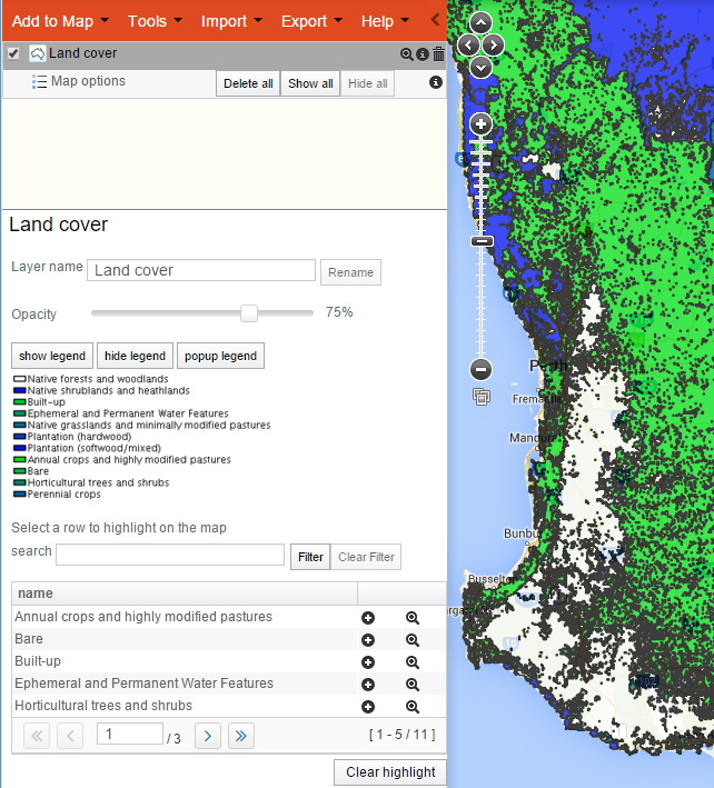
Contextual layer legend
The figure above shows the legend and part of the map for the land cover for Australia. There are 11 distinct classes, each with a corresponding colour on the legend and map. Unlike environmental layers, the contextual layers allow you to highlight one class on the map by clicking on the class name in the bottom part of the legend (call it the sub-legend). The highlight can be cleared by clicking on the Clear highlight button at the bottom of the sub-legend. This method using the legend is a quick way of scanning through the areas associated with legend classes. You can page through the various classes or search for a class by name.
If you want to create a new layer from one class of the contextual layer click on the plus symbol to the right of the class name. This method is a quick alternative to using ‘Add to Map | Areas |Gazetteer polygon’ and selecting the class name. This latter process works because all contextual layers classes have been entered into the ALA’s gazetteer database.
Layers that are automatically updated weekly
There are four layers that are recalculated weekly due to the additions of occurrence records
- Endemism (see Crisp et al. 2001)
- Edemism non-marine (see Crisp et al. 2001)
- Occurrence density and
- Species richness
Each of these values are calculated at global extent using a 0.1 degree (~10km) grid. It is likely that additional similarly derived layers will be added when we become aware of their potential utility. Suggestions always welcomed to support@ala.org.au.
Viewing all available layers in the Spatial Portal
A complete list of available layers with thumbnail images and metadata can be found at http://spatial.ala.org.au/layers. This list can also be downloaded as a Comma-separated variable (CSV) or JSON (JavaScript Object Notation) formats. See the links on the top of the page.
The Display Name contains a link to available metadata for each layer. The Short Name provides a shorcut for entering layer names in the Spatial Portal. For example, Bio01 can be used in place of “Bioclim Temperature – annual mean”.
NOTE: The list contains 400+ layers and can take many minutes to generate.

Layers list
References
Belbin, L., Williams, K.J. (2015). Towards a national bio-environmental data facility: experiences from the Atlas of Living Australia. International Journal of Geographical Information Science. http://dx.doi.org/10.1080/13658816.2015.1077962.
Crisp, M.D., Laffan, S., Linder, H.P. and Monro, A (2001). Endemism in the Australian Flora. Journal of Biogeography 28, 183-198.
Williams, K.J., Belbin, Lee, Austin, Michael P, Stein, J., Ferrier, S. (2012). Which environmental variables should I use in my biodiversity model? Special Issue of International Journal of Geographical Information Science, iFirst, 1–39. DOI:10.1080/13658816.2012.698015