Faceting and Filtering : ALA Support

Faceting

A facet is an a single attribute of a species that has been indexed against all species records in the ALA’s species database; an indexed attribute. In the Spatial Portal facet classes are rendered in the legend and on the map with different colours. In the Spatial Portal, one or more of the classes of the facet can be selected, and then filtered in or out, to create new point layers.

In the example below, the Atlas records have a facet called Institution and one of the classes in this facet would be Australian Museum. Occurrences that are part of this facet have been selected and coloured red.

Facet attributes by Category

The current list of contextual layer facet options includes:

————— Custom —————

Dataset
data_provider
Coordinate uncertainty (in metres)
Date (by decade)

————— Taxon —————

Scientific name
Scientific name (unprocessed)
Subspecies
Genus
Family
Order
Class
Phylum
Kingdom
Identified to rank
Name match metric
Lifeform
Common name (processed)
Species subgroups
Species interaction

————— Location —————

Country
State/Territory
CAPAD 2014 Terrestrial
CAPAD 2014 Marine
Estuary habitat mapping
Directory of Important Wetlands
National Dynamic Land Cover
Commonwealth Electoral Boundaries
IBRA 7 Regions
IBRA 7 Subregions
IMCRA 4 Regions
IMCRA Meso-scale Bioregions
Koppen Climate Classification (All Classes)
Land use
Local Government Areas
Geomorphology of the Australian Margin and adjacent seafloor
NRM Regions
RAMSAR wetland regions
River Regions
ASGS Australian States and Territories
States including coastal waters
Surface Geology of Australia
Vegetation – condition
el1076
Vegetation types – native
Vegetation types – present
Elevation
min_elevation_d_rng
Sensitive
Species habitats
Coordinate uncertainty (in metres)
Spatial validity
location_id

————— Identification —————

Identified by
raw_identification_qualifier
Taxon identification issue
Specimen type
original_name_usage

————— Occurrence —————

Collector
Sex
Life stage
Cultivation status
Month
Year
occurrence_decade_i
State conservation
State conservation (unprocessed)
event_id

————— Record —————

Record type
Multimedia
Presence/Absence

————— Assertions —————

Sensitive
Record issues
Outlier for layer
Outlier layer count
Has user assertions
Assertions by user
Associated records
Duplicate record type

————— Attribution —————

Atlas user
Dataset
dataset_name

When you choose a facet in the legend, a suite of coloured classes will be displayed below the layer list and map options. Each legend class can be selected or deselected using the checkboxes to the left of the class name. If there are a large number of classes, they will be paged. The ordering of the classes will be by decreasing number of occurrence records.

The following example shows occurrence data for all species within the current extent. It is faceted on Species name showing the occurrence points coloured by class. The species Platycercus elegans is selected using the facet class checkbox and all points of occurrence data for that species are highlighted with a red circle on the map.

Step 1: Open the spatial portal. Zoom and pan the area of interest.

Step 2: Add | Species - choose All species and ensure the area is restricted to the Current extent.

Note: once the occurrence points are displayed there will be a Facet option available. The default is User defined colour.

Step 3: Select to facet on Scientific name

Step 4: Select (tick) Platycercus elegans

How can faceting and filtering be used? Occurrence records could be, for example, separated into specific States, by LGA areas or by Record Issues.

Scatterplots also support faceting (but not filtering). For more information see Scatterplot faceting »

Filtering

Species occurrence records can be filtered on the basis of one or more facet classes. For example, you can select an existing point layer and then create a new point layer that contains records that have a date of >=2000 or you could create a new point layer that does not have any record issues. Note that with many of the facets, not all records will have that attribute recorded. For example, records may have a missing date.

For example, below is an example of Eucalyptus gunnii in Tasmania with the Facet ‘Year’ selected. Once one or more classes are selected (1989 and 1990 below for example), two buttons appear below the legend

‘Create layer with selection’. Pressing this button creates a new point layer that will include only the selected records.
‘Create layer without selection’. Pressing this button creates a new point layer that will contain all records but the selected records.

In the example below, the new layer has been renamed to make it obvious that it contains only records from the years 1989 and 1990.

This image shows all occurrences of Eucalyptus Gunnii with a layer created for all occurrences recorded in 1989 and 1990 (circled).

Unticking the layer of all occurrences will show you just the 1989 and 1990 recorded occurrences layer.

Filtering on ‘Data Quality’ issues (‘Fitness for use’)

A common task before any analyses of data is to ensure that the data is ‘fit for use’. To achieve this, we use a category of facets (see above) called ‘Assertions’. When any data is entered into the ALA, even when it is imported for use in one session (see Import | Points), a large suite of automated tests are run against each record (see http://biocache.ala.org.au/ws/assertions/codes).

Any test that results in some form of warning or error will be reported as an ‘assertion’. For example, if there is no date value in a record, the assertion will be “incompleteCellectionDate”. The description here is standardized in what is called camelCase – the text will start with lower case and where the first letter or any subsequent words are capitalized as in “thisIsAnExampleOfCamelCase”. The meaning is usually (hopefully) clear.

The classes in the Assertion category are

Sensitive (records that have some sensitivity flag associated)
Record issues (all values of tests/assertions)
Outlier for layer (which environmental layers have occurrence records that are outliers)
Outlier layer count (how many of the 5 environmental layers have outlier records)
Has user assertions (records that have been annotated by one or more users)
Assertions by user (which users have annotated the records)
Associated records
Duplicate record type (the nature of the differences in suspected duplicate records)

Let us take a practical example using the species Vulpes vulpes.

Step 1:

Map the occurrence records of the fox Vulpes vulpes - Add to map | species| Vulpes vulpes. At time of writing, there were 70 249 records. The first thing to note is that there are records in Germany, Italy and Japan.

Note: that there are also 2 records that have not been coded by country. Selecting the Not Supplied value allows you to see the occurrences appear to be in Japan.

Step2:

Filter out the non-Australian records. This can be done by:

Choose the Facet Country
Selecting the tick box beside Australia and clicking on Create layer with selection
OR
Choose the Facet Country
Click on Germany, Italy, Japan and Not supplied tick boxes and selecting Create layer without selection

Take your pick but the first is easier here. The result will be a be a new layer. This layer should be renamed to something like “Vulpes vulpes – Australia” to make it clear what this new point layer contains.

Step3:

Select the new layer Vulpes vulpes – Australia (make sure the original layer, Vulpes Vulpes (World) is unticked)

Select the facet Record issues on the Australian records. You will see that there are plenty of records with issues that we may want to remove (filter out) from the Australian records.

Select those issues you want to remove by checking the tick boxes beside them. What you select will depend on your knowledge of the data and the issues that have been raised by the automatic tests. I have selected a range of issues that would disqualify records from many analyses.

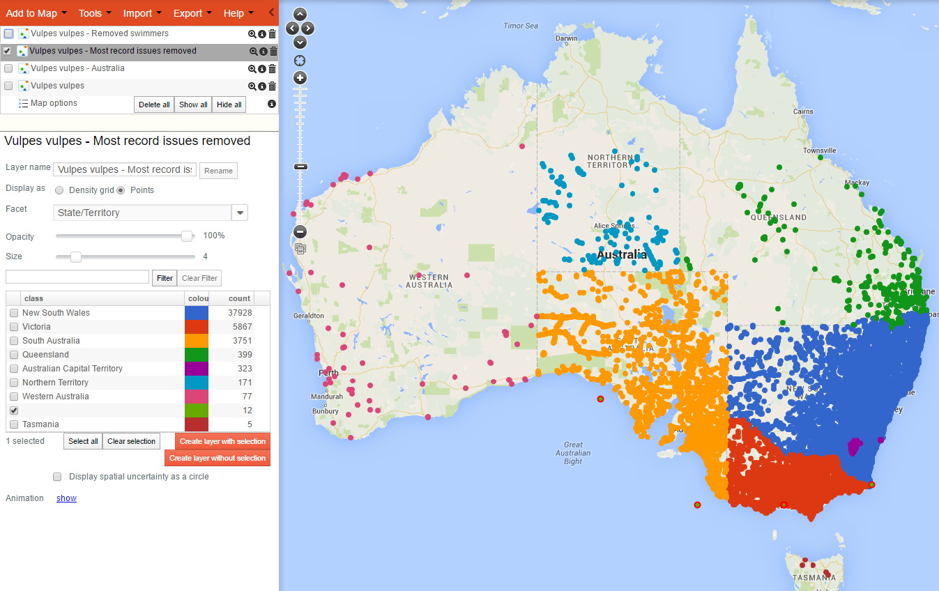
Once the classes have been selected, click on Create layer without selection and a new filtered points layer will be selected that do not have any of the selected issues. Name this layer something like Vulpes vulpes – Australia - Most issues removed.

Vulpes vulpes records with some obvious record issues

Step 4:

If you now deselect the previous point layer so only the last filtered layer is displayed on the map, you will see that we still have issues!

The most immediate issue is that we have foxes that appear to have been sighted swimming. In some cases, this may be genuine, but it is obvious that some have been badly geolocated or there has been some transcription problem with the latitudes and longitudes. The quickest way to deal with this problem is to select States and Territories in the drop-down list for the legend of the last filtered layer.

We can easily see that 12 records do not occur in any State or Territory, and those points have been highlighted on the map. You can zoom and pan the map to see the issues if desired. In many cases, the accuracy or precision of the locations are likely problems. In the former for example, the coordinates may have been wrongly read from a map, while the latter can be caused by not having sufficient number of decimal places to place the observation on land. When ready, click on ‘Create layer without selection’ to create a new point layer of Vulpes vulpes without ‘swimmers’!

Vulpes vulpes filtered for swimmers!

Vulpes vulpes filtering for swimmers!

We now have a dataset that should be more reliable but a quick examination of the map of the distribution of the records in the new point layer (named above as “Vulpes vulpes – Removed swimmers”), it is obvious that there is a bias by State and Territory. The records in South Australia and the Northern Territory seem to largely stop at the Western Australian border. Ditto, Queensland records look a little suspicious. Foxes are smart, but not that smart? What you do next will depend on what you plan to use the data for. I have scanned the map and noted that while there were no ‘Sensitive records’, those in Victoria look very much like they are largely on a regular grid. Does this imply the the records were forced onto a regular grid or, less likely, that the records were part of a systematic survey? There is nothing specific in the Victoria records I examined to suggest spatial displacement, but I have not checked thoroughly. You may need to. If the record locations have been moved onto a grid, you need to figure out if that invalidates an analysis? The points appear to be on roughly a 10km grid. Will this change the environmental associations – unlikely given the spatial distribution of foxes in Australia – they are almost everywhere. It would be easier to figure out where they are least likely to be. More on that issues below!

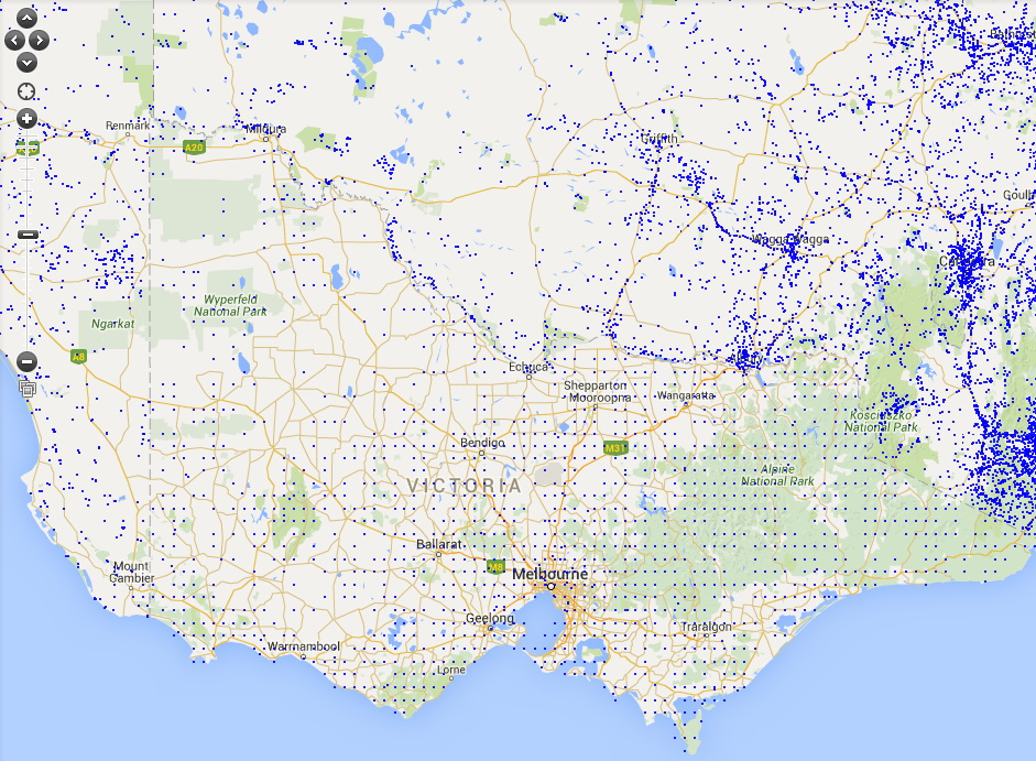
Gridded records in Victoria?

To check some records, click on the (i) button to the right of the layer name. This links to the metadata about these records, but in this case, we want to look at the Victorian records – so click on the link “Table view of these records”. This takes us into what is called the biocache – the general part of the ALA dealing with records (not the Spatial Portal). What you will see on the left-hand side of the window is the same facets as in the Spatial Portal, and they can be used in the same way. Also note that at the top of the window you will see the filters applied to the original Vulpes vulpes records. There is nothing specific in the Victoria records I examined to suggest spatial displacement, but I have not checked thoroughly. You may need to.

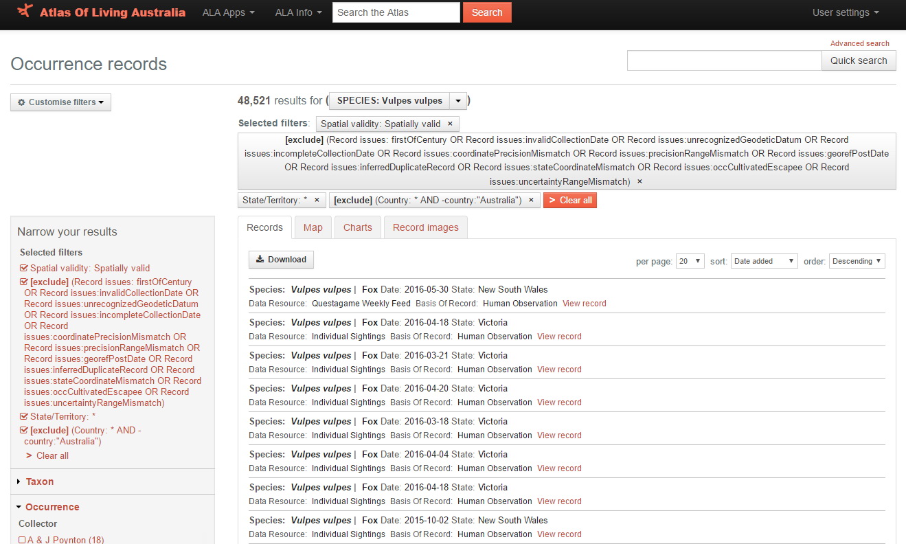
Filtered records in the biocache

At this point, you can view the records by clicking on them, or you could carry on filtering the data by other attributes. For this exercise, I will see if I can find any suspect records on the basis that foxes don’t like being far from water. I will do a scatterplot (menu Tools | Scatterplot in the Spatial Portal – which will likely be on the tab of your browser to the left) and use two environmental map layers that may identify issues
- Distance – to permanent water (weighted) and
- Aridity index – annual mean

and this is what we will see

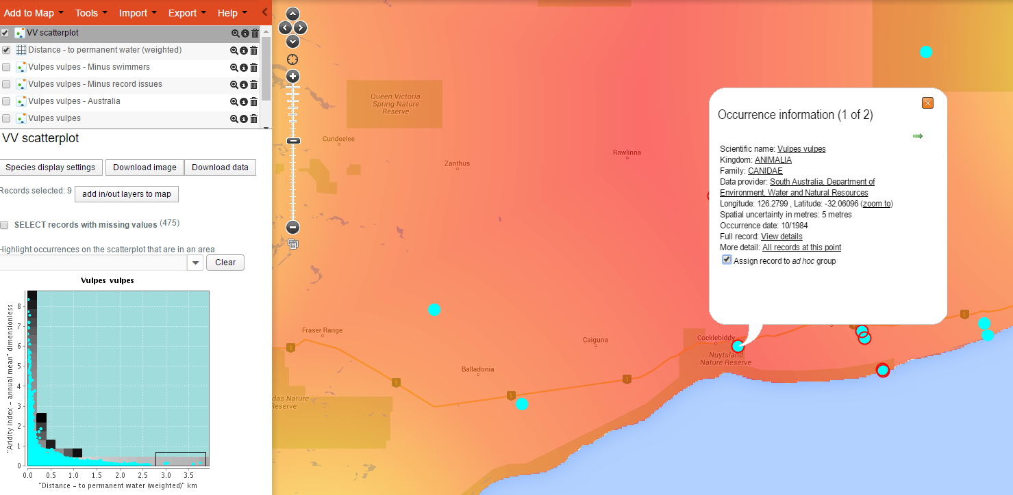
Filtering records by assigning them to an ad hoc group

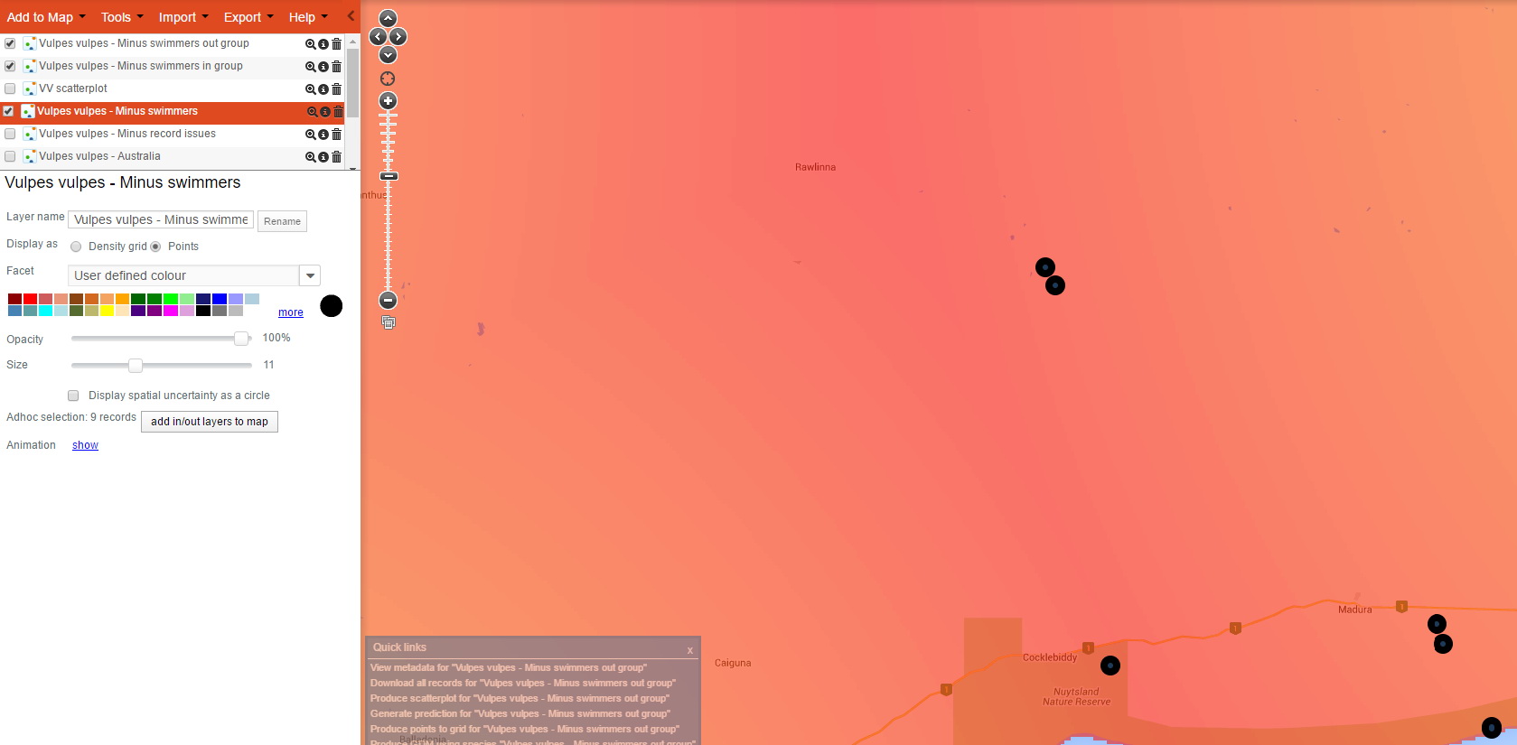
I selected the points that you can see on the far right of the scatterplot (drag a bounding box over the points to be selected) – sighting of foxes that were a maximum distance to permanent water – and those points have been identified on the map with a red ring around them. There are 9 that seem to be outliers on these criteria (aridity and distance to permanent water). If you then click back to the point layer “Vulpes vulus – minus swimmers” and then click on each of the suspect points you will get a pop-up window with an option down the bottom to assign them to an “ad hoc group” (you will need to click the light blue arrow on the pop-up to get to all the points in a cluster).
If you then click on the button beneath the legend “Add in/out layers to map”, two new point layers will be created, one with ONLY those selected points (in group) and one that OMITS those 9 selected points (out group). It is the latter that you then may want to use in analysis.

Filtering out ad hoc points

We now have a somewhat ‘cleaned’ dataset that could be used for various analyses. To ensure we can always get back to this filtered dataset, we again click on the metadata icon next to the layer “Vulpes vulpes – minus swimmers out group” and click on the bottom link to view these records in the biocache.

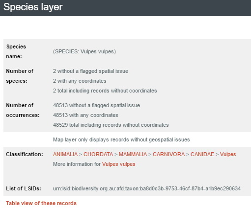
Point layer metadata

Note the URL (the web address) in your browser is giving you an address that you can use if you wish to return to these records or even download these records. In this case the URL is http://biocache.ala.org.au/occurrences/search?q=qid:1467001326172. The “qid” is the unique identifier for these records. If you wanted to say download all these records, just including species name, latitude and longitude, you could use this web address: http://biocache.ala.org.au/ws/occurrences/index/download?q=qid:1467001326172&reasonTypeId=1. This says to the ALA, the reason I downloaded this data is “Biosecurity management/planning”. The downloaded zip file will contain a citation file, a headings file, a data file and a read me file. The data file will contain the species name, latitude and longitude and any assertions that have at least one TRUE flag against any of the records.

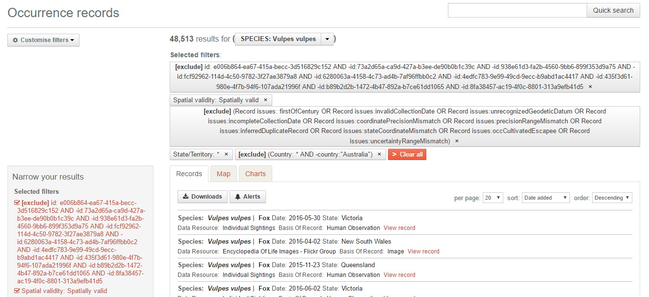
Filtered data in biocache

Faceting in Scatterplots

Legends in the Spatial Portal allow the user to modify the display of the mapped layer. For more information on Legends »

Legends in the scatterplot function operate slightly differently to those of standard layers. Manipulating the legend for a Scatterplot not only effects the points on the map (geographic), but the points on the Scatterplot (environmental) graphical display as well.

To activate the legend in the Scatterplot, click on the ‘Species display setting’ button. This creates a floating window that renders changes to the points in both spaces on the basis of selected legend properties. The user has to press the ‘Apply’ button to activate the changes. Again, faceting is one of the options.

Note: Filtering by facet classes is not available. Scatterplots have the ability to create new layers based on records within or without defined environmental boundaries, but not based on contextual attribute values of the records themselves. For more information on Scatterplots »

In the image below the Scatterplot is faceted on ‘Basis of Record’.