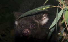
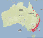
Ecologists, field naturalists and all sorts of people might ask such a question. The greater glider, Petauroides volans (Kerr, 1792), is Australia's largest glider, an arboreal marsupial that feeds on Eucalyptus leaves at night and shelters in tree hollows during the day. We have records of where it has been observed, but where else might it be? Species distribution models are often used to answer such questions.
By Jane Elith, University of Melbourne, School of Botany

Greater Glider – Petauroides volans
- Where should I hunt next for this rare orchid?
- Which areas are most suitable for restoration, for this endangered turtle?
- What is this fish species responding to? – is it light, depth, currents, or what?
- Where are suitable climates for this bird, and how might these climates change?
- What parts of my state are most climatically similar to other places where this invasive ant thrives?
The Atlas of Living Australia provides the infrastructure necessary for making a species distribution model. This is a Case Study on the Greater Glider using the Atlas web site.
Species Distribution Modelling and Maxent
There are many ways to make a species distribution model. The ALA has chosen MaxEnt as its modelling method because it suits most of the current data, works well, is fast, and is freely available. You can run MaxEnt within the ALA interface, or you can download the program and run it on your own computer. The Atlas has a wide range of species data and over 300 environmental layers. To run MaxEnt on your computer, you would need the species data (downloadable from the Atlas) and relevant environmental data (which is harder to find, download and use).
MaxEnt compares environments where the species occurs to those in the broader landscape. It finds the model that best emphasizes the environments occupied by the species whilst also predicting new places where there are no records. MaxEnt runs automatically in the Atlas, but can be “tweaked” more if run on your computer. In the Atlas, the key choices are:
What records to include
When you map the species occurrences, some may be wrong (e.g. plants in the sea, or mountain species in a desert). Your first job is to get rid of any obvious errors.
What layers to use
Models will be most sensible and best at predicting when the environmental variables (“layers”) that are selected are most relevant to the species. Don’t use them all! Pick a subset that you believe are best related to the environment where the species occurs.
How to define the landscape
MaxEnt compares the location of occurrences with environments across the area selected. In the Atlas, this area is called the Active Area, and by default is the displayed map window extent. This may not be optimal. If you want to work out why your species is south of the divide rather than north, in Victoria, you won’t want the model to use all of Australia because it would be making too broad a comparison. You can define the Active Area in one of eight ways.
Modelling the Greater Glider

Greater Glider distribution
Ecologists say that the greater glider needs the right climate and other resources to satisfy their energy and water requirements as they feed, move around, reproduce, and rear young. These must include suitable tree hollows for shelter. We selected 13 layers that are likely to represent those conditions – either directly, for the glider itself, or indirectly, by providing suitable conditions for the trees it requires. The layers were humidity (annual), precipitation (of driest and wettest months), temperature (maximum of the hottest month, minimum of the coldest month, mean annual maximum), substrate (lithology fertility, organic carbon, topographic wetness, soil depth), topography (topographic relief, valley bottom flatness index) and vegetation (NDVI mean).

Active area selection
Interpreting the Results
We used two models because we chose two landscapes. Both predicted similar distributions, and used similar variables with similar response shapes to predict the distribution. It is not always like this – quite often, the important variables will change depending on the scale of the landscape used. The figures below are for the all-Australia landscape. They show the mapped predicted distribution, with green values higher probabilities than oranges. The four graphs show the fitted functions for the four most important variables: from left to right: precipitation of the driest month; mean annual relative humidity; maximum temperature of the hottest month and precipitation of the wettest month. The percentages below each graph show the relative importance of the variable in the model. The shapes of the graphs show the species response to that variable when the other variables in the model are held constant. For example, the first graph shows that the species is unlikely to occur when the driest month is very dry (i.e. towards the left end of the x axis). These graphs give insights into the variables most strongly related to the species distribution. These should be checked against ecological knowledge.

Greater Glider modeling
What could go wrong? Pitfalls for the unwary
These models, like all, are based on certain assumptions. If these aren’t met, your model might be nonsense. The most common problems are with the species data: the assumption is a random sample, so if you have, instead, a very biased sample (e.g. if only one state was surveyed) then the model will be more a model of sampling effort than species distribution. Or if the taxonomy is unclear and you have records for 3 species rather than one, then your model will be trying to predict suitable conditions for all three species. Or if you have very few records (e.g. less than 30), there won’t be much information to train the model on. Perhaps you might also lack the relevant predictors, or the species might be mostly restricted by the distribution of a predator. All of these have solutions, but will need some extra work on your desktop version. Similarly, using these models for climate change or invasive species predictions is rather more difficult than for species at equilibrium, and needs special care.
About the author

Author Jane Elith
Contributors to this page

The University of Melbourne School of Botany
Referenced links
Scientific References
Elith, J. and Leathwick, J.R., 2009. Species distribution models: ecological explanation and prediction across space and time. Annual Review of Ecology, Evolution and Systematics, vol. 40, pp. 677-697.
Pearson, R.G., 2007. Species’ distribution modeling for conservation educators and practitioners. American Museum of Natural History – Download pdf
Franklin, J., 2010. Mapping Species Distributions: Spatial Inference & Prediction. Cambridge University Press, UK.
Kearney, M.R.; Wintle, B.A. and Porter, W.P., 2010. Correlative and mechanistic models of species distribution provide congruent forecasts under climate change. Conservation Letters, vol. 3, pp. 203-213.
Phillips, S.J., Anderson, R.P. and Schapire, R.E., 2006. Maximum entropy modeling of species geographic distributions. Ecological Modelling, vol. 190, pp. 231-259.
Phillips, S.J. and Dudík, M., 2008. Modeling of species distributions with Maxent: new extensions and a comprehensive evaluation. Ecography, vol. 31, pp.161-175. Download pdf.
Elith, J., Phillips, S., Hastie, T., Chee, Y., Yates, C. and Dudik, M., 2011 in press. A statistical explanation of MaxEnt for ecologists. Diversity and Distributions